|
|
|
|
|
|
Capacitor standardisation using a reference inductor.
David W Knight
|
1. Introduction. 2. Background. |
3. Initial capacitor calibration. >>> Not finished. |
|
Abstract: A solenoid wound with thin wire and having a large pitch / wire-diameter ratio can be used as a radio frequency reference inductor, provided that the operating frequency range is such that the length of the winding wire never exceeds 60 electrical degrees. When the wire diameter is small relative to the solenoid diameter, and the spacing between turns is relatively large, dispersion due to the proximity effect is negligible. Dispersion due to the skin effect is however significant for thin wire, but this can be modelled accurately. Hence, presuming that there is no magnetic core, that losses in the dielectric of the coil-former are small, and that the dispersion region around the SRF is avoided; it becomes possible to correct for all known non-idealities of the inductor to an accuracy of better than 1 part in 104. A quasi-ideal lumped-element inductor, realised by applying mathematical corrections to the behaviour of an actual inductor, can be used to standardise small capacitors to a precision of a few femto Farads. A method is demonstrated whereby the uncertainties in a set of reference capacitors are aggregated in a manner which produces new nominal values of greatly increased precision. |
|
1. Introduction: If a measurement procedure produces a result in such a way that the statistical noise is apparent (i.e., if there is some variability in the result beyond a certain number of significant digits), then it is possible to improve the precision of the measurement by repeating it several times and taking the average. If the number of measurements is n, then the standard deviation of the average is given by the standard deviation of a single measurement divided by √n. When the same measurement is repeated several times, the individual results can be regarded as samples taken from a single parent population. The averaging process improves the precision because the sample mean tends towards the parent mean as the number of samples increases. It is possible to treat samples from different parent populations as though they belong to the same parent population, provided that some rule which relates the various populations is known. Such is the case when data are subjected to a weighted regression procedure, the weighting factor serving to scale the individual error distributions so that they become identical. In this way, the statistical advantage which accrues from repeating a single measurement can be obtained from a set of disparate measurements, provided that the scaling rule can be accurately defined. It is well known that the inductance and the so-called 'self-capacitance' of an inductor can be determined by measuring the parallel resonant frequency against a series of reference capacitances. For such an experiment, to a degree of approximation to be discussed in detail shortly, the resonant frequency is given by the expression: f0 = 1 / { 2π√[L (C0 + Cref)] } Where Cref is the applied reference capacitance, and C0 is the sum of the strays and the self-capacitance of the coil. After rearrangement, the resonance formula becomes: Cref = -C0 + 1/[ (2πf0)² L ] This is a straight-line graph of the form y=a+bx, where the independent variable x might be chosen as (say) 1/(2πf0)², to find the gradient b=1/L and intercept a=-C0. The problem with the linear regression procedure for finding L and C0 however, is that it only gives a statistically convincing outcome when the accuracy of measurement is relatively poor. If we assume that all of the experimental error is confined to the determination of the reference capacitances; a satisfactory outcome of a reduced χ² test applied to the data will typically only be obtained if the uncertainty in the capacitance measurements is of the order of several percent. An improvement in accuracy will show that the straight-line graph is not straight after all, the discrepancy being due to the assumption that L and C0 are constants. An inductor operating at radio frequencies can only be fully understood as a transmission-line device. It stores energy by virtue of the fact that it takes a finite time for electromagnetic radiation to travel the length of the winding wire. This is a very different picture to that given by lumped-component theory, which is based on the conception that the dimensions of electrical devices are negligible in comparison to the wavelength. That the inductor, in particular of all circuit components, does not fit into the latter regime should be obvious; and so self-capacitance is primarily a model parameter, which serves to extend lumped element theory to moderately high frequencies; but does not wholly exist for static electric fields, and does not necessarily predict the self-resonant frequency (SRF). Hence the first requirement, prior to proposing that an inductor can be used to provide a scaling rule for the comparison of capacitors of differing values, is to establish the extent to which the lumped component model is valid. Part of the answer to this question lies in the solution of Maxwell's equations for the Ollendorf sheath-helix model, which has received much discussion over the years (see, for example [18], [19] and references for Inductor self-resonance . . . ). The theory shows that the apparent velocity for electromagnetic propagation along the helix varies with frequency; and that it does so in a particularly non-linear manner around the SRF. The lumped component model is only accurate insofar as the apparent inductance vs. frequency curve that it produces corresponds to that of a dispersive short-circuited transmission line. This observation might seem to put an end to the idea of making use of the 'linear' relationship mentioned above, except for an ideosyncracy of the mathematics. The impedance-related properties of cylindrical objects are given by combinations of Bessel functions (also known as 'cylinder functions'). The resulting mathematical description is that of systems for which changes of behaviour can have a relatively rapid onset. For an inductor, it transpires that the lumped component model is accurate over a large interval and then suddenly breaks down. Theory and data indicate that the representation of a solenoid as a lumped inductance in parallel with a lumped capacitance works until the length of the conductor exceeds about 60 electrical degrees. Further difficulties exist however, the problem being that the idealised sheath helix on which the transmission-line theory is based is not physically realisable. Thus, presuming that we have the good sense to eliminate permeability dispersion by not using a magnetic core, and that we eliminate permittivity dispersion by using a low-loss coil-former; we must still take into account two remaining dispersion phenomena, these being the skin effect and the proximity effect. Most people interested in electromagnetism are aware of the proximity effect as a frequency-dependent increase in the electrical resistance of coils beyond that due to the skin effect. The principle of causality demands however, that an increase in losses is always followed by a reduction of reactance; which means that the proximity effect must be associated with inductance variation. It is possible to rationalise this decline in inductance as a reduction in the effective diameter of the solenoid; there being a tendency, in wire of finite diameter, for the current to crowd in the region closest to the coil axis at high frequencies. It follows that the amount of variation can be controlled by choosing a wire diameter which is small relative to the diameter of the solenoid. Thin wire, of course, is not optimal when designing inductors for high Q, but the issue here is to obtain constant inductance. For the standardisation technique to be described; a solenoid of 48.7mm diameter wound with 0.15mm diameter wire was used. This limits the inductance variation due to the proximity effect to a factor of: (48.7 - 0.15) / 48.7 = 0.9969 i.e., the maximum possible variation, neglecting end effects which will limit it further, is about 3 parts in 1000 (0.3%). Although a constancy of external inductance to within 0.3% is good, it is still not good enough for the purposes of this study. Hence some additional measure which precludes the maximum variation from occurring is required. The solution is to use a large winding-pitch to wire-diameter ratio; i.e., to minimise the proximity effect by maintaining a relatively large distance between adjacent turns. An empirical study of the proximity effect in solenoids was carried out in 1947 by R G Medhurst [Medhurst 1947]. Results were given in the form of a table of proximity factors, in the high-frequency limiting case, for solenoids of varying length / diameter and pitch / wire-diameter ratio ( |
|
Notice that the AC resistance is increased by a factor of 5.8
when there is no spacing between the turns (p/d=1), but the proximity
effect has all but died out when p/d=10. For the work to be reported,
coils were wound on a grooved former of 0.1" (2.54mm) pitch,
with a wire diameter of 0.15mm. This gives p/d=17. The value
in the table for p/d=10 (the largest p/d ratio reported) is 1.03,
and so, from the shape of the curve, we might reasonably expect
Ψ to be about 1.01 for the test coils; i.e., the increase
in AC resistance due to the proximity effect will be about 1%. The variation of AC resistance, of course, does not necessarily quantify the corresponding variation of inductance. It is reasonable to assume however, that only a small fraction of the 0.3% possible variation in inductance will actually occur. As a rough estimate, we can say that the variation will be about 1% of 0.3%; i.e., about 3 parts in 100 000. This is well below the statistical noise of the measurements to be reported. Although the use of thin wire eliminates the proximity effect, it has the effect of moving the most dispersive region of internal impedance into the radio-frequency range. This precludes the use of thick-conductor approximations for AC resistance and internal inductance, and thereby presents a computational challenge. The problem is that the exact calculation of internal impedance involves the use of Kelvin Bessel functions of large argument. Due to computer rounding errors, the calculation of these functions using series expansions fails in the radio-frequency range when modelling the skin-effect in thin wires. The use of polynomial approximations is an alternative [14], but none of the resulting formulae are continuous. Also, the very high accuracy obtainable by piecewise application of discontinuous formulae is not actually needed. Hence a companion study was undertaken with a view to obtaining simple continuous formulae of accuracy sufficient for inductor modelling [see: Zint.pdf]. The outcome was a formula for AC resistance accurate to within 0.16%, and a formula for internal inductance accurate to within 0.07%. Internal inductance is most important here, because AC resistance is required only for a very minor correction to the resonant frequency. For the inductors and frequency ranges used in this study, the maximum internal inductance contribution to the total inductance is about 1%. Hence the inaccuracy in the internal inductance formula used gives an overall maximum error contribution of 0.12% of 1%; i.e., about 1.2 parts in 100 000. One final source of possible inductor non-ideality is the existence of multiple-reflection resonances. The true (fundamental) SRF of an inductor (as opposed to the inaccurate extrapolated SRF predicted by the 'self capacitance') occurs when the physical length of the winding wire is close to λ/2. This can be understood by considering a wave reflecting between the impedance discontinuities which occur at the inductor terminals, parallel resonances occurring at frequencies where a wave arrives back at its starting point in phase with itself. It follows that there will be an infinite number of alternating series and parallel resonances (overtones) above the SRF; but what is less often recognised is that there can also be fractional harmonics, particularly when the electrical length of the wire is λ/2n [20]. These multiple-reflection resonances are generally weak, but can be detected by placing a high-Q inductor in a radio-frequency field and picking-up the scattering signal using a loop or an electrometer probe. The implication is that there will be a weak aperiodic cyclical variation in the impedance appearing at the inductor terminals; and the question arises as to whether the steps taken to eliminate all of the other sources of model error will allow these undulations to stand out from the experimental noise. An educated guess says not, but some insurance against systematic error is warranted. The solution adopted here is to repeat the capacitor comparison several times, using a different number of turns on the coil-former in each case, and to take the average result. In this way, any minor impedance variations will be smeared out (regardless of the cause). Another reason for repeating the data acquisition is that it gives a method for finding the experimental noise level. The procedure of interest here is that of comparing a set of fixed capacitors of differing value. On producing a regression line, there will be a difference between the nominal and the calculated values for each capacitance. This will be true even if one or more of the capacitors is a laboratory standard, the reason being that a standard is nothing more than a capacitor for which the value is known to greater than usual precision. The use of weighting factors ensures that the better-known capacitances are taken more seriously than the less well known; but even the calibration of a good standard can be improved by comparing it against a large number of inferior standards. Hence, after an experimental run, the calculated value for a particular capacitor is a better estimate of its true value than was its original nominal value. The problem however, is that if we change the capacitor values to agree with their new estimates and refit the data, the new fit will show no noise whatsoever and we will have lost all knowledge of the experimental uncertainty. The solution is to repeat the experiment several times and take the average, in which case the noise will reappear and standard-deviations can be estimated. The various experimental runs can, of course, be made using the same inductor; but it is far better to alter the inductor in some sequential manner and thereby also cancel any low-level systematic errors. |
|
2. Background: The experiment to be described was devised in order to exploit an opportunity created by the purchase of about 100 close-tolerance capacitors. The point is to make use of the fact that a set of n electrical components each having a known relative uncertainty δ in its nominal value posesses a collective uncertainty δ/√n; provided that the errors are normally distributed, and provided that it is possible to scale the individual measurements in such a way as to normalise their means and standard deviations. The capacitors were obtained for the purpose of making plug-in reference capacitances, to be used primarily for the determination of inductor self-capacitance by the linear regression method described earlier. The reason for adopting a set of fixed capacitors, rather than using a variable reference, was that writing down the value of a previously measured capacitor would be much quicker than an earlier used method; which involved adjusting a trimmer capacitor and then unplugging it and transferring it to a measuring bridge. The fixed capacitors moreover, all being physically small and of similar dimensions, have parasitic inductance which is minimal, relatively easy to calculate, and fairly consistent across the whole set. Since the capacitors were to be used in the production of data to be fitted to a regression line; it seemed natural to use the same regression procedure to standardise them. That this could be done (and perhaps had to be done) became obvious after performing a few self-capacitance determinations using their initial calibration values. When evaluating a linear regression procedure, there is usually little point in plotting a graph of the regression line itself. It will look like a straight line wilth data points adhering closely to it, and little insight will be gained. Far more interesting is the graph of residuals (nominal value minus calculated value), which shows the experimental noise. The reduced χ² test, which tells whether the linear relationship is plausible, is well and good; but it is the overall appearance of the noise graph which tells the experimenter whether of not the scatter is truly random. Any curvature due to systematic error is usually immediately obvious; but for the experiments in question, it was the appearance of pseudo-randomness which attracted attention. Apart from known sources of curvature, such as internal inductance and velocity dispersion; the graphs produced did appear to be random when considered individually. When compared however, they all looked similar; i.e., the same 'random' pattern was being produced by every experiment. Hence the graphs were not showing experimental noise, but a set of points corresponding to the deviation of the known value of a given reference capacitor from the far better estimate given by combining the uncertainties of of all of the capacitors. Thus it was discovered that the somewhat high level of experimental noise associated with using variable reference capacitors had been suppressed, only to show up the calibration errors in the fixed capacitors. This led to the idea of recalibrating the fixed capacitors by comparing each one against the whole set, and thereby refining the experimental procedure. To do that however, would require a quasi-perfect inductor for reference. Hence the deliberations relating to the design of RF reference inductors, as outlined in the previous section. |
|
3. Initial capacitor calibration: The capacitors to be compared were silvered-mica units in the range 2.2 to 220pF, with nominal tolerances of ±1% or ±0.5pF whichever is greater. They were supplied in lots of five of each value, and totalled about 100, although a few other similar capacitors from other sources were added to the collection. Mica is a natural material of variable composition, which means that a capacitor made using it has to be tested and trimmed after construction. This makes it impossible for the manufacturer to skimp on materials by supplying units which are biased in value towards the lower tolerance limit (a potential problem with rolled-foil capacitors for example). Hence, for a set of mica capacitors, presuming that the manufacturer's standards are correctly maintained; the true values will be scattered randomly around the nominal values and there will be no deliberately-introduced systematic error. The tolerances quoted for manufactured parts are usually guaranteed or 'brick wall' limits. Presuming that the manufacturing process is relatively imprecise and that there is no systematic error in the production sampling, this means that the most probable difference between the nominal value and the actual value will be about half the tolerance. For samples taken from a normally distributed population, the most probable error is one standard deviation (1σ). Hence, for a given capacitor, the standard deviation of its nominal value can be taken to be about half its tolerance. All of the capacitors were measured using a laboratory bridge operating at 1.5915MHz. The estimated standard deviation (ESD) for bridge measurements, determined by spot calibration using 0.1% secondary standards, was about ±0.5% ±0.05pF. The measurements were found to be consistent with the hypothesis that all of the capacitors were within tolerance to a probability of about 95% (2σ), although one capacitor was rejected for having an unusually high ESR. Taking the 1σ uncertainties of the initial nominal values to be 0.5% or 0.25pF, whichever is greater (i.e., half the tolerance); the manufacturer's value was combined with the measured value in each case, weighted according to the relative uncertainty, to produce a new nominal value. Note that the bridge measurement is the better estimate for the smaller capacitances, but that the manufacturer's value is the better estimate for the larger capacitances. Overall, without exaggerating the accuracy of the evaluation, all of the capacitances were taken to be known to within ±0.5% ±0.05pF (ESD) after this initial establishment of working nominal values. It was not the intention to use all of the capacitors for coil experiments, but to select the sample closest to the average from each set of five nomininally identical units; the average being taken to represent to the nominal value according to the manufacturer's standard. In this way, a single example of each of the preferred values supplied was selected and subsequently mounted on a plug-in header. Of the capacitors left over, some were also made up into series or parallel combinations, to fill-in gaps in the sequence; their deviations from the average of the preferred-value group being used to deduce the nominal value of the composite in combination with re-measurement on the bridge. Prior to the initial measurements, the leads of all of the capacitors were splayed-out in the manner required for mounting. For soldering to the plug-in header, the leads of the selected capacitors were trimmed slightly and wrapped around the header pins. Careful measurements on some of the smaller value capacitors could find no significant difference in capacitance before and after mounting (within a few femtoFarads). Hence the amount of stray capacitance lost by trimming the wires was taken to be about the same as that gained due to the pins and the plastic spacer. By relating the measurement to the average of a set of 5; the standard deviation of the value of a chosen capacitor is effectively reduced by a factor of about 1/√5, i.e., 0.45. Hence, bearing in mind that the bridge measurement is dominant for small-value capacitors, the tolerances of the finally mounted reference capacitors were estimated to be ±0.23% ±0.05pF. This corresponds to an expression for the standard deviation of a given capacitance: σ = √[0.05² + (0.0023C/pF)²] [pF] and the weighting coefficient for least-squares fitting is 1/σ² (the reciprocal of the variance). The absolute weightings so determined (purely from consideration of manufacturer's tolerances and bridge measurements) were found to return reduced χ² (goodness of fit) values close to unity in subsequent data reductions using reference inductors; confirming the statistical reasoning up to this point. |
|
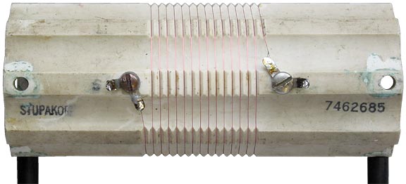
4. Apparatus. After the initial calibration, the capacitors were used to make a number of self-capacitance determinations on small toroidal inductors [see 'Self-capacitance of toroidal inductors']. It was during the course of that work that the pseudo-random pattern of residuals was noticed; superimposed on a background of minor non-linearities attributable primarily to the dispersive nature of the magnetic core material, skin and proximity effects, and the transition to the limiting helical phase velocity on the approach to the SRF. Thus, although it was evident that the capacitor calibration could be improved, it was also recognised that it would not be possible to do so on the basis of the data then available. Hence a solenoid inductor, of thin wire, with wide spacing between the turns, was wound on a ribbed and grooved ceramic coil-former of World War II vintage made by the Stupakoff Ceramic & Manufacturing company of Pennsylvania. This was mounted on plastic stand-off pillars, 10cm above a wooden bench and connected to the test jig used for the toroidal inductor measurements. The connection was by means of a pair of 10cm long, 1.6mm diameter copper wires. Shown below is the coil-former fully populated with 15 turns of wire. . |
|
spreadsheet: refcoil_1.ods
. spreadsheet: refcoil_Cstd.ods . Correlation. The error in a calibrated value is always correlated with the error in the standard against which the calibration is made. Hence, in a mutual calibration of this type, although the accuracy is greatly increased, there will always be some correleation between the uncertainties in the various capacitor values. |
References
|
[14] "Numerical calculations
of internal impedance of solid and tubular cylindrical conductors
under large parameters" W. Mingli and F. Yu (Northern
Jiaotong University, School of Electrical Engineering, Beijing,
China). IEE Proceedings, Generation, Transmission and Distribution.
January 2004, Vol 151, Issue 1, p. 67-72. [18] "Theory of the Beam-Type Traveling-Wave Tube". J R Pierce. Proc. IRE. Feb. 1947. p111-123. See Appendix B, p121-123, "Propagation of a wave along a helix", which gives Schelkunoff's derivation of propagation parameters for the Ollendorf sheath-helix. [19] "Coaxial Line with Helical Inner Conductor". W Sichak. Proc. IRE. Aug. 1954. p1315-1319. Correction Feb. 1955, p148. [20] Radio Frequency Transistors, Norm Dye and Helge Granberg. Motorola inc. / Butterworth Heinemann, Newton MA. 1993. ISBN 0-7506-9059-3 Line-length resonance: p142. |
© D W Knight 2008.
David Knight asserts the right to be recognised as the author of this work.
|
|
|
|
|
|